Nearest neighbor regularization for decision trees
Here we describe a new way to regularize decision trees which outperforms conventional pruning. Optimizing the regularization parameter is also more straightforward. We assume a nodding acquaintance with decision trees and their training.
A Julia notebook showing the testing reported here is also available.
Decision trees in supervised learning
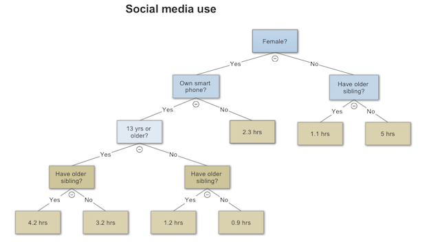
Regression and classification algorithms based on ensembles of decision trees - e.g., random forests and extreme random forests - are popular because they are easy to implement, robust to outliers, and handle mixed data types. They also perform competitively using default values for their tuning parameters. Although not as accurate, a single decision tree has the advantage that the prediction algorithm is exceedingly simple to describe, which is important in some applications.
Pruning
In practice, a single decision tree invariably overfits the
data and requires regularization. The most common form of
regularization is pruning based on leaf size: Unless the number of
training patterns reaching a tree node exceeds a certain a preset size
(the regularization parameter, here called min_patterns_split) then
the node is not split further, becoming a leaf (prediction node) whose
prediction is the mean value of the target for patterns reaching the
node. For the sake of concreteness, we are assuming here our problem is a
regression problem, rather than a classification one.
Nearest neighbor regularization
The parameter min_patterns_split takes on discrete
values $ 2, 3, 4\ldots$. In the method we call nearest neighbor
regularization, the regularization parameter is continuous. Here’s how
the algorithm works:
-
Fit a decision tree to the training data as usual, with no pruning (
min_patterns_split=2). -
Choose a non-negative number $r<1$; this will determine the degree of regularization.
-
With $r$ fixed, the model’s prediction on an input pattern $P$ is determined as follows:
-
Run the pattern $P$ down the tree as usual, until you reach a prediction node $N_0$ and let $p_0$ be the target value for the single pattern that reaches $N_0$ during training (the usual unregularized prediction).
-
Label the nodes visited along the way using reverse-order indices. So, the stump node will be $N_d$, where $d$ is the depth of $N_0$, which is followed by $N_{d-1}, N_{d-2},\ldots,$ and so on, until we reach the last nodes visited, $\ldots, N_3,N_2,N_1,N_0$.
-
At each node $N_j$ branch to the node that is not $N_{j+1}$. So, if the decision criterion at $N_j$ applied to $P$ says branch left, then branch right instead, and vice-versa. Thereafter, continue branching as usual, arriving a new final node $L_j$ different from $N_0$ (unless $j=0$). We may think of $L_j$ as the “$j$th closest leaf to $N_0$”, as measured by pattern $P$, and let $p_j$ denote the prediction there (the target value for the single training pattern reaching $L_j$).
-
The regularized prediction for pattern $P$ is then a normalized weighted sum of the predictions of the “nearby” leaves: \[ p = \frac{1}{s} \Big(\,p_0 + r p_1 + r^2 p_2 + r^3 p_3 + \cdots + r^d p_d\,\Big). \] Here $s$ is the sum of the weights: \[ s = 1 + r + r^2 + r^3 + \cdots + r^d = \frac{1-r^{d+1}}{1-r}. \] For large datasets one may want to truncate the sums to some maximum depth to speed up prediction.
-
-
Now that predictions are defined for our regularized model, we can compute errors and tune the regularization parameter $r$ as usual, comparing errors on a holdout validation dataset, or using cross-validation.
Tests
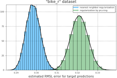
We compare nearest neighbor regularization with regular pruning on six real datasets. Further details on the datasets are given at the end.
For each dataset a root-mean-square (RMS) or root-mean-square-log
(RMSL) error is used as the criterion for tuning the regularization
parameters min_patterns_split (for pruning) and $r$ (for nearest
neighbor regression).
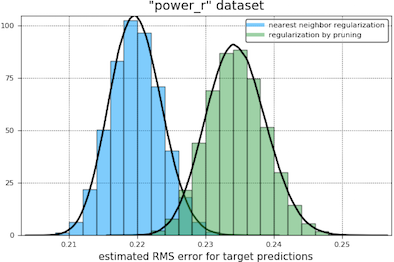
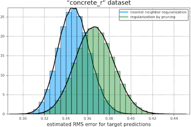
In our first comparison of the regularization methods we obtain bootstrap histograms of 12-fold cross-validation errors for each tuned model, presented on the same plot. Our results are shown below. The light blue curve appears to the left of the green when nearest neighbor regularization is performing better.
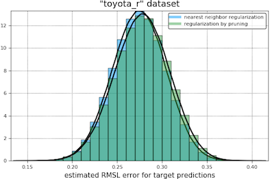
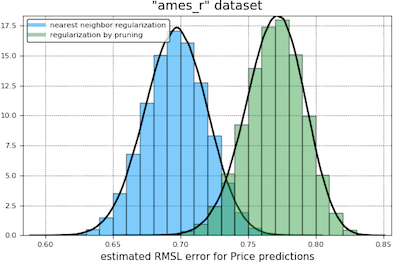
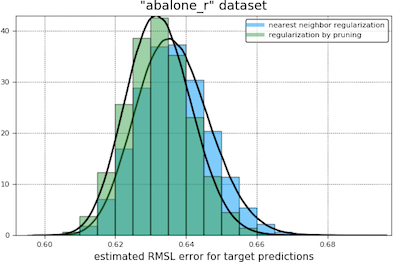
In our second comparison, we had the two types of regularization compete in a two-sided student t-test, treating the cross-validation errors as independent samples of the expected error of a trained and tuned model (the null hypothesis being that this error is the same for both types of regularization). At a coverage of 95% in these tests, nearest neighbor regularization beats pruning in every case except the “toyota_r” and “abalone_r” datasets, where the outcome is a draw.
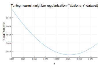
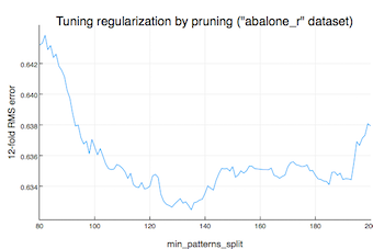
Ease of optimization
We found the nearest neighbor regularization
parameter $r$ (always between 0 and 1) easier to tune than the
pruning parameter min_patterns_split. The plots below, shown for the
“abalone_r” dataset, give an indication of this:
Data sources
The datasets were chosen ahead of time, without prior knowledge of how well the regularization methods would compare. We did rule out some very large datasets, to reduce testing time. The table below gives further details.
| Handle | Full Name | No. Input Attributes | No. Instances | Source |
|---|---|---|---|---|
| “bike_r” | Bike Sharing* | 11 | 1739 | [1] and UCI Machine Learning Repository |
| “toyota_r” | Toyota Corolla | 9 | 1436 | [2] and Data Illuminations |
| “ames_r” | Ames House Price Data** | 12 | 1456 | [3] and Kaggle |
| “abalone_r” | Abalome (seafood) | 8 | 4177 | [4] and UCI Machine Learning Repository |
| “power_r” | Combined Cycle Power Plant | 4 | 9568 | [5,6] and UCI Machine Learning Repository |
| “concrete_r” | Concrete Compressive Strength | 8 | 1030 | [7] and UCI Machine Learning Repository |
*Year information and the season field have been dropped, while the date has been replaced by the sine and cosine of the corresponding within-year phase $\theta$ (so that $\theta=0$ corresponds to January 1st, and $\theta=\pi$ corresponding to the middle of the calendar year).
**With a reduced set of features selected by a tree-based ranking scheme.
References
[1] Fanaee-T, Hadi and Gama, Joao, “Event labeling combining ensemble detectors and background knowledge”, Progress in Artificial Intelligence (2013): pp. 1-15.
[2] Original source unknown, but referenced on this blog of Peter Chan, San Diego.
[3] De Cock, Dean, “Ames, Iowa: Alternative to the Boston Housing Data as an End of Semester Regression Project”, Journal of Statistics Education Volume 19, Number 3(2011).
[4] Warwick J Nash, Tracy L Sellers, Simon R Talbot, Andrew J Cawthorn and Wes B Ford, “The Population Biology of Abalone (Haliotis species) in Tasmania. I. Blacklip Abalone (H. rubra) from the North Coast and Islands of Bass Strait”, Sea Fisheries Division, Technical Report No. 48 (1994), ISSN 1034-3288.
[5] Pınar Tüfekci, Prediction of full load electrical power output of a base load operated combined cycle power plant using machine learning methods, International Journal of Electrical Power & Energy Systems, Volume 60, (Sept. 2014), Pages 126-140.
[6] Heysem Kaya, Pınar Tüfekci , Sadık Fikret Gürgen: Local and Global Learning Methods for Predicting Power of a Combined Gas & Steam Turbine, Proceedings of the International Conference on Emerging Trends in Computer and Electronics Engineering ICETCEE 2012, pp. 13-18 (Mar. 2012), Dubai.
[7] I-Cheng Yeh, “Modeling of strength of high performance concrete using artificial neural networks,”Cement and Concrete Research, Vol. 28, No. 12, pp. 1797-1808 (1998).